2  Descriptive Statistics

3 Mean versus median

3.1 Variance

x <- c(97.88, 107.91, 88.26, 115.21, 87.38)

\[ s^2 = \frac{\Sigma(x_i - \bar{x})^2}{n - 1} \tag{3.1}\]

variance_vis(x, plot_deviances_x = 4, plot_deviances = FALSE, plot_population_variance = FALSE) +
    ylim(c(-1, 5)) + theme(axis.text.y = element_blank()) +
    annotate('text', x = mean(x) + (max(x) - mean(x)) / 2, y = 4,
             label = bquote("x - bar(x)"), parse = TRUE, vjust = 1.5, size = 8)

Figure 3.1: Deviation for the largest value.

variance_vis(x, plot_deviances_x = 4, 
             plot_deviances = 4, 
             plot_population_variance = FALSE) +
    ylim(c(0, 20))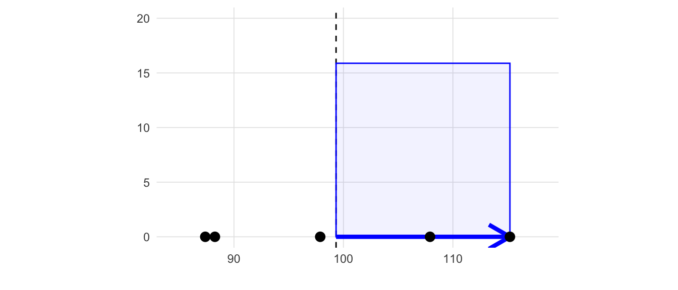

Figure 3.2: Squared deviation for the largest value.

variance_vis(x, 
             plot_deviances = TRUE, 
             plot_population_variance = FALSE) +
    ylim(c(0, 20))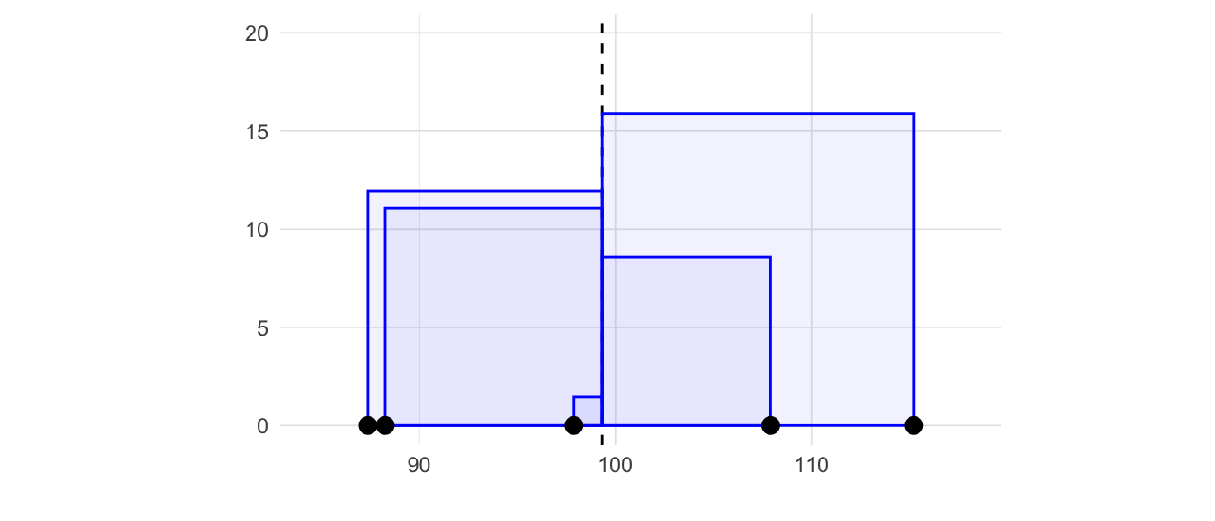

Figure 3.3: Squared deviation for all observations.

variance_vis(x, 
             plot_deviances = TRUE, 
             plot_population_variance = TRUE,
             plot_sample_variance = TRUE) + 
    ylim(c(0,35))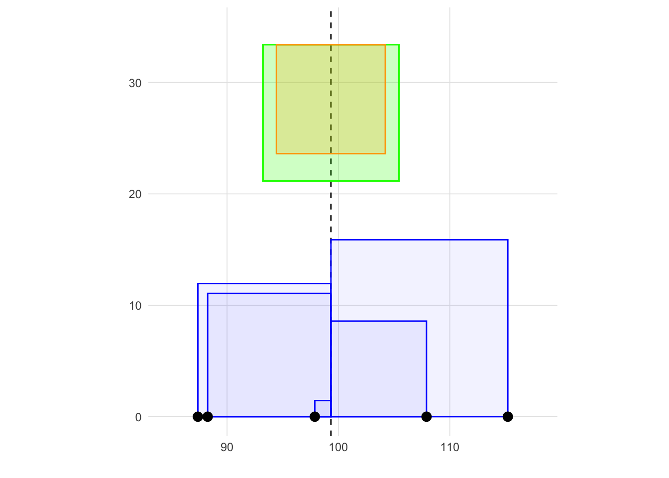

Figure 3.4: Squared deviation for all observations along with population and sample variances.

\[ s = \sqrt{s^2} = \sqrt{\frac{\sigma(x_i - \bar{x})^2}{n - 1}} \tag{3.2}\]

3.1.1 Sample versus population variance

We used the population variance above because the denominator, N, is easier to demonstrate since the variance is simply the average of the area of all the squares. However, we will almost always want to estimate the sample variance which changes the denominator to n - 1 (technically called the degrees of freedom which will be described in more detail in later chapters). In fact, the var function in R to calculate variance will always return the sample variance (and sd function for standard deviation by extension). In practice reporting the sample variance when working with a population can be considered a slightly conservative estimate. However, as n increases, the difference between the sample and population variances are going to converge (see Appendix A for more details about convergence, limits, and core calculus concepts helpful for learning statistics).

Let’s first define two function to caclulate the sample and population variances.

sample_var <- function(x) {
    mean_x <- mean(x)
    n <- length(x)
    sum( (x - mean_x)^2) / (n - 1)
}

population_var <- function(x) {
    mean_x <- mean(x)
    N <- length(x)
    sum( (x - mean_x)^2) / N
}

We will now calculate the sample and population variance from a vector randomly generated from the normal distribution with mean of 0 and standard deviation of 1.

max_n <- 500
x <- rnorm(max_n)
variances <- data.frame(n = seq(2, max_n, 1),
                        sample_var = numeric(max_n - 1),
                        population_var = numeric(max_n - 1))
for(i in seq_len(nrow(variances))) {
    n <- variances[i,]$n
    variances[i,]$sample_var <- sample_var(x[1:n])
    variances[i,]$population_var <- population_var(x[1:n])
}
variances <- variances |>
    dplyr::mutate(Difference = abs(population_var - sample_var))

Figure @ref(fig:fig-variance-convergence) depicts the two variances along with the difference for sample sizes rangine from 2 to 500. The blue line representing the difference is very close to zero when n = 200.

variances |> 
    reshape2::melt(id.vars = 'n', variable.name = 'Estimate', value.name = 'Variance') |>
    ggplot(aes(x = n, y = Variance, color = Estimate)) +
        geom_path()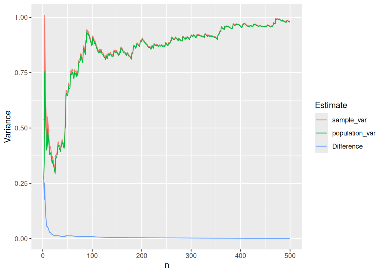

Figure 3.5: Sample versus population variances as n increases.

Examining the last five rows (i.e. n = 496 to 500) show that the difference in the two variances is less than 0.01.

tail(variances, 5)

      n sample_var population_var  Difference
495 496  0.9842646      0.9822802 0.001984404
496 497  0.9836034      0.9816243 0.001979081
497 498  0.9827055      0.9807322 0.001973304
498 499  0.9811142      0.9791481 0.001966161
499 500  0.9792802      0.9773217 0.001958560

This Shiny application can be run locally using the VisualStats::variance_shiny() function.