9  Multiple Regression

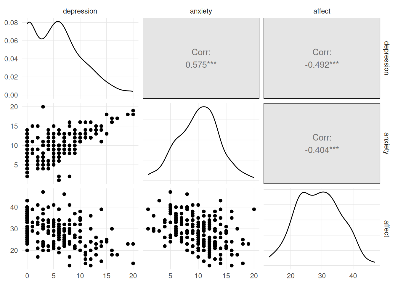
Now that we have defined the relationship between two variables using ordinary least squares regression, we want to extend that framework to include omre variables. Multiple regression is the procedure used to predict an outcome (i.e. dependent variable) from two or more independent variables. We are going to use the depression data set which includes baseline measures from 200 individuals who participated in psychological intervention (Boswell, n.d.). We can visually represent these data using a 3d scatter plot where our dependent variable is on the z-axis and independent variables are on the x and y-axes.

multiple_regression_vis(y = depression$depression,
                        x1 = depression$anxiety,
                        x2 = depression$affect,
                        y_lab = 'Depression',
                        x1_lab = 'Anxiety',
                        x2_lab = 'Affect',
                        plot_regression = FALSE,
                        plot_residuals = FALSE)

Algebraically we represent this model as:

\[Y_{depression} = B_0 + B_{anxiety} X_{anxiety} + B_{affect} X_{affect}\]

We now have two slopes (coefficients) to estimate In the OLS regression chapter we defined the slope of the line as the product of the correlation and the ratio of the standard deviations. We might be tempted to estimate the two slopes using:

\[ B_{anxiety} = r_{depression,anxiety} \frac{S_{depression}}{S_{anxiety}} \]

\[ B_{affect} = r_{depression,affect} \frac{S_{depression}}{S_{affect}} \]

However, this would be incorrect because anxiety and affect are correlated.

GGally::ggpairs(depression[,c('depression', 'anxiety', 'affect')])

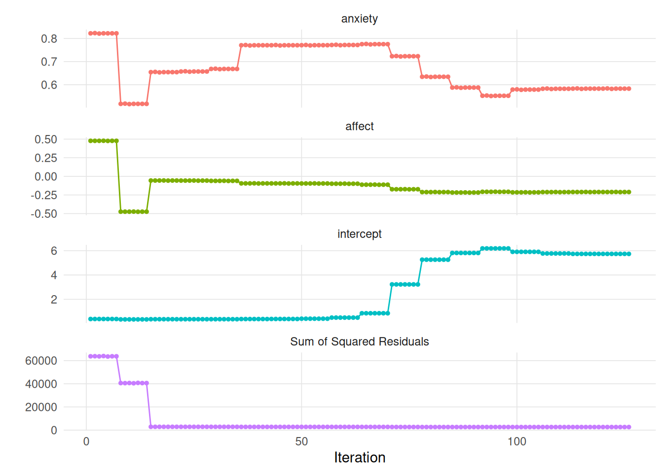
Although it is possible to estimate the slopes using a closed form solution, it requires knowledge of matrix algebra which is beyond the scope of this book. Instead, to explore multiple regression visually, we will use maximum likelihood estimation. Our goal, like OLS, is to minimize the sum of squared residuals. The following function generalizes the calculation of the sum of squared residuals introduced in the maximum likelihood estimation for an arbitrary number of independent variables.

residual_sum_squares <- function(parameters, predictors, outcome) {
    if(length(parameters) - 1 != ncol(predictors)) {
        stop('Number of parameters does not match the number of predictors.')
    }
    predicted <- 0
    for(i in 1:ncol(predictors)) {
        predicted <- predicted + parameters[i] * predictors[i]
    }
    predicted <- predicted + parameters[length(parameters)]
    residuals <- outcome - predicted
    ss <- sum(residuals^2)
    return(ss)
}

We can then use the optim_save function to find the combination of slopes and intercept that minimizes the sum of squared residuals.

optim.rss <- optim_save(
    par = runif(3),
    fn = residual_sum_squares,
    method = "L-BFGS-B",
    predictors = depression[,c('anxiety', 'affect')],
    outcome = depression$depression
)

summary(optim.rss)

3 parameters estimated in 126 iterations.
Final parameter estimates: 0.583, -0.21, 5.736

plot(optim.rss, param_labels = c('anxiety', 'affect', 'intercept'), result_label = 'Sum of Squared Residuals')

The regression results can then be written algebrically as:

\[ Y_{depression} = 5.74 + 0.58 X_{anxiety} + -0.21 X_{affect} \]

The figure below adds the plane estimated to the 3d scatter plot. The vertical lines going from each point to the plane represent the residuals.

multiple_regression_vis(y = depression$depression,
                        x1 = depression$anxiety,
                        x2 = depression$affect,
                        y_lab = 'Depression',
                        x1_lab = 'Anxiety',
                        x2_lab = 'Affect',
                        plot_regression = TRUE,
                        plot_residuals = TRUE)

Multiple regression uses the same lm function to estimate the model, we simply add our additional independent variables.

lm_out <- lm(depression ~ anxiety + affect, data = depression)
summary(lm_out)

Call:
lm(formula = depression ~ anxiety + affect, data = depression)

Residuals:
   Min     1Q Median     3Q    Max 
 -7.43  -2.26  -0.27   2.66   8.31 

Coefficients:
            Estimate Std. Error t value Pr(>|t|)    
(Intercept)   5.7364     1.6676    3.44  0.00071 ***
anxiety       0.5830     0.0776    7.52  1.9e-12 ***
affect       -0.2105     0.0405   -5.19  5.2e-07 ***
---
Signif. codes:  0 '***' 0.001 '**' 0.01 '*' 0.05 '.' 0.1 ' ' 1

Residual standard error: 3.7 on 197 degrees of freedom
Multiple R-squared:  0.411, Adjusted R-squared:  0.405 
F-statistic: 68.8 on 2 and 197 DF,  p-value: <2e-16

9.1 Interaction Effects

multiple_regression_vis(y = depression$depression,
                        x1 = depression$anxiety,
                        x2 = depression$affect,
                        y_lab = 'Depression',
                        x1_lab = 'Anxiety',
                        x2_lab = 'Affect',
                        plot_regression = TRUE,
                        plot_residuals = FALSE,
                        interaction = TRUE)

lm_out_2 <- lm(depression ~ anxiety * affect, data = depression)
summary(lm_out_2)

Call:
lm(formula = depression ~ anxiety * affect, data = depression)

Residuals:
   Min     1Q Median     3Q    Max 
-8.118 -2.487 -0.265  2.315 10.027 

Coefficients:
               Estimate Std. Error t value Pr(>|t|)    
(Intercept)    -8.41373    3.53037   -2.38    0.018 *  
anxiety         1.87034    0.29608    6.32  1.8e-09 ***
affect          0.24870    0.10933    2.27    0.024 *  
anxiety:affect -0.04303    0.00958   -4.49  1.2e-05 ***
---
Signif. codes:  0 '***' 0.001 '**' 0.01 '*' 0.05 '.' 0.1 ' ' 1

Residual standard error: 3.5 on 196 degrees of freedom
Multiple R-squared:  0.466, Adjusted R-squared:  0.458 
F-statistic:   57 on 3 and 196 DF,  p-value: <2e-16